Creating a distance cartogram using OSM data

Introduction

We are looking to build a unipolar distance cartogram (also called a centered time cartogram) using only data from OpenStreetMap (OSM): it is going to use both geographic layers describing the territory and travel time data from OSM.

This type of cartogram visualizes travelling times from a reference starting location to other destinations in a selected area. In the resulting map, the geographic distance are replaced by time distance and the underlying map layers are deformed accordingly.

This highlights the use of several packages developed at RIATE, including:

mapsf to create maps with sf objects,
osrm for calculating distance-time matrices from OSM data,
maposm to easily retrieve OSM data (this is a wrapper around osmdata),
distanamo for creating distance cartograms.

Installing and importing packages

mapsf and osrm are available both on CRAN and on riatelab’s r-universe while distanamo and maposm are only available from riatelab’s r-universe.

As a result, we propose to install all the packages from r-universe:

repos <- c("https://riatelab.r-universe.dev", "https://cloud.r-project.org")

install.packages("mapsf", repos = repos)
install.packages("osrm", repos = repos)
install.packages("distanamo", repos = repos)
install.packages("maposm", repos = repos)

Once installed, we can import the necessary packages:

library(sf)
library(mapsf)
library(osrm)
library(maposm)
library(distanamo)

Fetching OSM data

We are now retrieving OSM data for the study area of our choice: here we are interested in the accessibility (by bike, but we will see this later) from the market hall of Chambéry.

Let’s get the coordinates of the address of Chambéry’s market hall and then fetch the data for a radius of 3000 meters around it:

bb <- osmdata::getbb("10, Place Georges Clemenceau, 73100 Chambéry, France")
lon <- mean(bb[1, ])
lat <- mean(bb[2, ])
res <- get_city(c(lon, lat), r = 3000)
#> Getting buildings: 16.926 sec elapsed
#> Getting green areas: 1.723 sec elapsed
#> Getting water bodies: 2.761 sec elapsed
#> Getting roads: 1.247 sec elapsed
#> Getting streets: 2.111 sec elapsed
#> Getting railways: 0.35 sec elapsed

We can see that the resulting object is a list of sf layers:

print(names(res))
#> [1] "circle"   "green"    "water"    "railway"  "road"     "street"   "building"
#> [8] "urban"

Depending on the radius defined in the maposm::get_city function the result list contains either individual buildings (if r <= 5000) or urban patches (if r > 5000). As a result we need to filter the resulting list to remove any possible NULL entry:

res <- res[!unlist(lapply(res, is.null))]

Defining a reference point

We need to define a reference point from which the travel times will be computed. Since we used the address of Chambéry’s market hall as a center point to fetch the data, we can use the center of the circle that includes all the data:

start <- st_centroid(res$circle)

Sampling points

We then need a set of destinations to compute the travel times to. To do so, we sample roughly 200 points on the road network:

x <- st_sample(rbind(res$road, res$street), size = 200, type = "regular")
# x <- st_sample(res$road, size = 200, type = "regular")
points <- st_sf(id = seq_along(x), geom = x)
plot(st_geometry(points))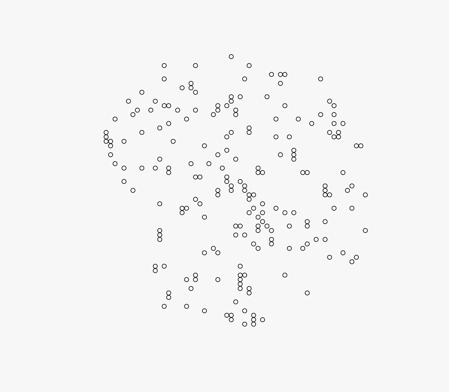

Making a map of the result

mf_map(res$circle, col = "#f2efe9", border = NA, add = FALSE)
mf_map(res$green, col = "#c8facc", border = "#c8facc", lwd = .5, add = TRUE)
mf_map(res$water, col = "#aad3df", border = "#aad3df", lwd = .5, add = TRUE)
mf_map(res$railway, col = "grey50", lty = 2, lwd = .2, add = TRUE)
mf_map(res$road, col = "white", border = "white", lwd = .5, add = TRUE)
mf_map(res$street, col = "white", border = "white", lwd = .5, add = TRUE)
mf_map(res$building, col = "#d9d0c9", border = "#c6bab1", lwd = .5, add = TRUE)
mf_map(res$circle, col = NA, border = "#c6bab1", lwd = 4, add = TRUE)
mf_map(start, pch = 23, col = "red", cex = 2, add = T)
mf_map(points, add = T, col = "blue")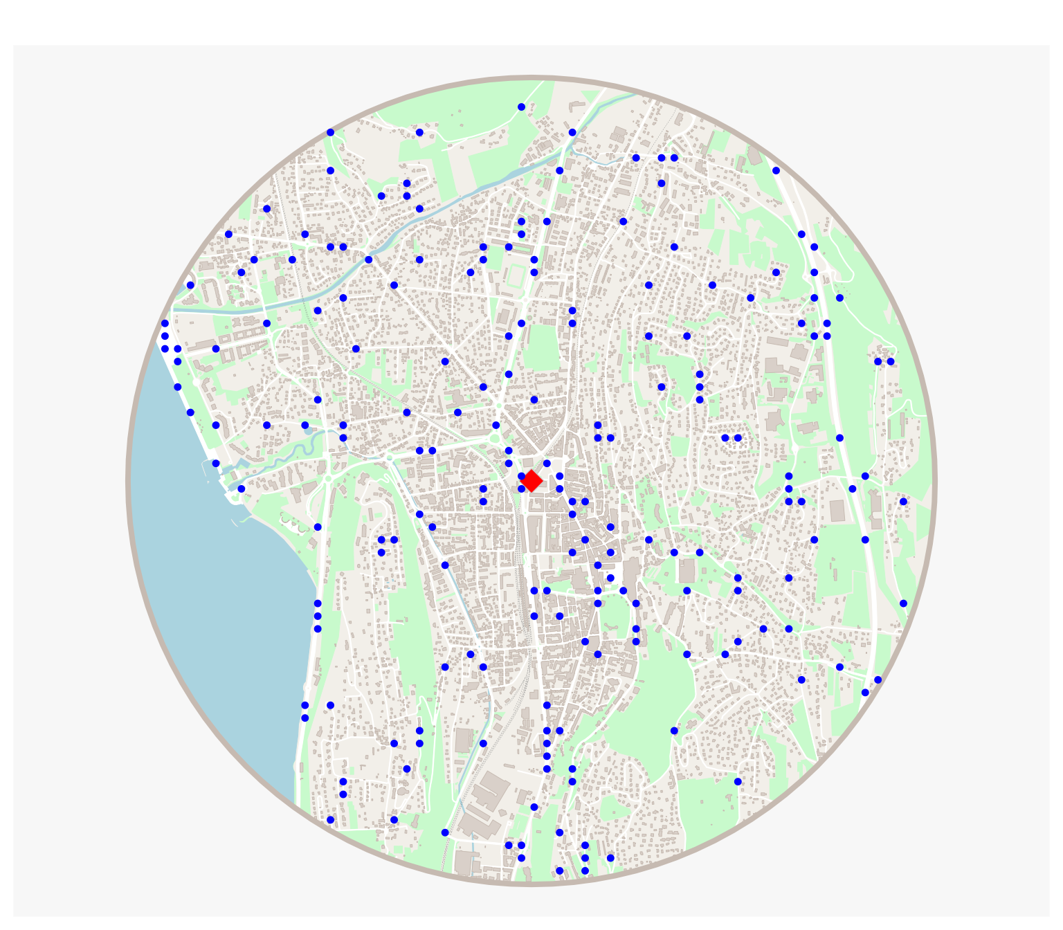

Computing travel times between the reference point and the sampled points

To do so, we can use the osrmTable function from the osrm package:

mat <- osrmTable(
  dst = start,
  src = points,
  osrm.profile = "bike"
)

points$durations <- mat$durations

Alternative to OSRM for computing travel times

Alternatively, if having a Valhalla instance under the hand and if the data preparation step included elevation data, you can also use it to compute travel times and benefit from taking the elevation into account:

library(valhallr)

s <- as.data.frame(st_coordinates(st_transform(start, "EPSG:4326")))
names(s) <- c("lon", "lat")

d <- as.data.frame(st_coordinates(st_transform(points, "EPSG:4326")))
names(d) <- c("lon", "lat")

durs <- sources_to_targets(
  s,
  d,
  costing = "bicycle",
  hostname = Sys.getenv("VH_HOSTNAME"),
  port = Sys.getenv("VH_PORT")
)

points$durations <- durs$time / 60

Note that we use environment variables to store the hostname and port of the Valhalla instance because this is our private instance. You need to replace Sys.getenv('VH_HOSTNAME') and Sys.getenv('VH_PORT') by the actual values you want to use.

Computing the positions of image points

We can now compute the positions of the image points using the dc_move_from_reference_point function. It takes as input the reference point, the other points, and the column name of the travel times in the other_points object.

This function will move the points by computing the reference speed (the average distance / time) and then moving the points further or closer to the reference point depending on the travel time to reach them.

pos_result <- dc_move_from_reference_point(
  reference_point = start,
  other_points = points,
  duration_col_name = "durations"
)

We can call the summary function to obtain a summary of the resulting object:

summary(pos_result)
#> Summary of the unipolar displacement result:
#> Min displacement: 0.4697282 [m] 
#> Mean displacement: 485.8294 [m] 
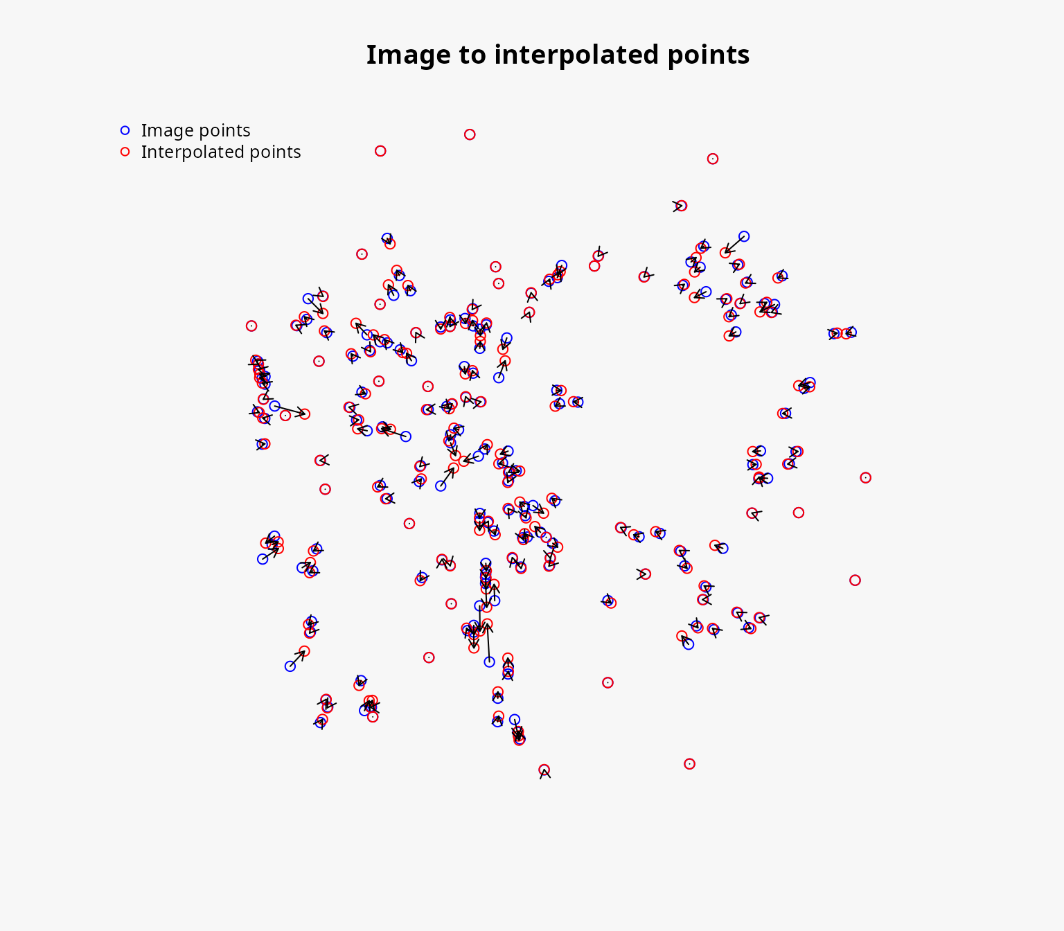
#> Max displacement: 1978.529 [m]

We can also plot the resulting object to visualize the positions of the image points and how they have been moved:

plot(pos_result)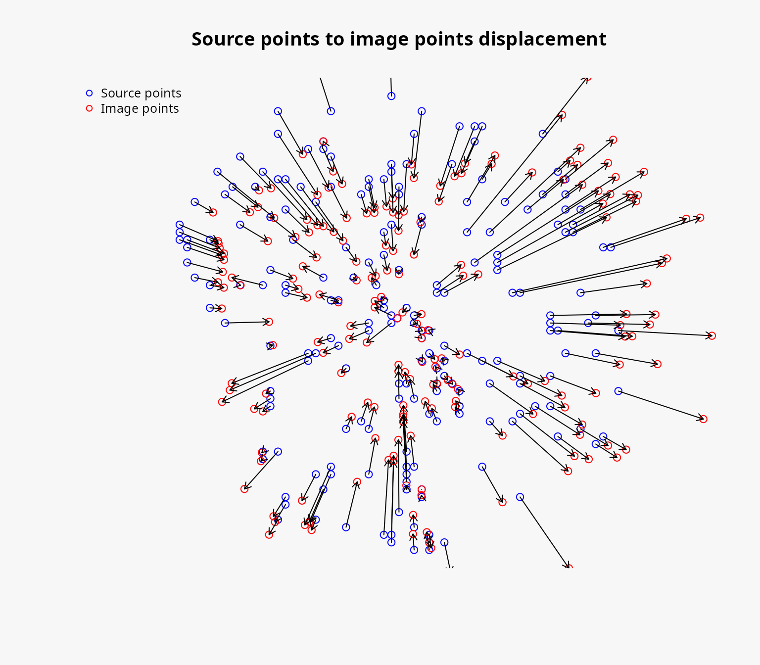

Creating the concentric circles

Since the cartogram will replace the geographic distance by time distance we can create concentric circles to represent the time distance from the reference point. Internally, this is possible because the reference speed has been stored in the resulting object of the dc_move_from_reference_point function.

The steps parameter is a list of the time distances we want to represent in the cartogram, in the same unit as the travel times (here, minutes).

circles <- dc_concentric_circles(
  pos_result,
  steps = list(5, 10, 15, 20)
)
circles
#> Simple feature collection with 4 features and 1 field
#> Geometry type: LINESTRING
#> Dimension:     XY
#> Bounding box:  xmin: 652762.2 ymin: 5726235 xmax: 662957.4 ymax: 5736430
#> Projected CRS: WGS 84 / Pseudo-Mercator
#>   step                       geometry
#> 1    5 LINESTRING (659134.2 573133...
#> 2   10 LINESTRING (660408.6 573133...
#> 3   15 LINESTRING (661683 5731333,...
#> 4   20 LINESTRING (662957.4 573133...

Creating the distance cartogram

We first need to compute the bounding box of all the layers we want to deform using the interpolation grid to ensure that the interpolation grid covers the whole area of interest.

bbox <- dc_combine_bbox(res)

We can then create the interpolation grid:

The precision parameters controls the size of the grid cells (higher is more precise, for example 0.5 generally gives a coarse result, 2 a satisfactory result and 4 a particularly fine result). A precision of 2 is usually a good default value and this is what we choose to use here.

igrid <- dc_create(
  source_points = pos_result$source_points,
  image_points = pos_result$image_points,
  precision = 2,
  bbox = bbox
)

Various information can be obtained from the interpolation grid:

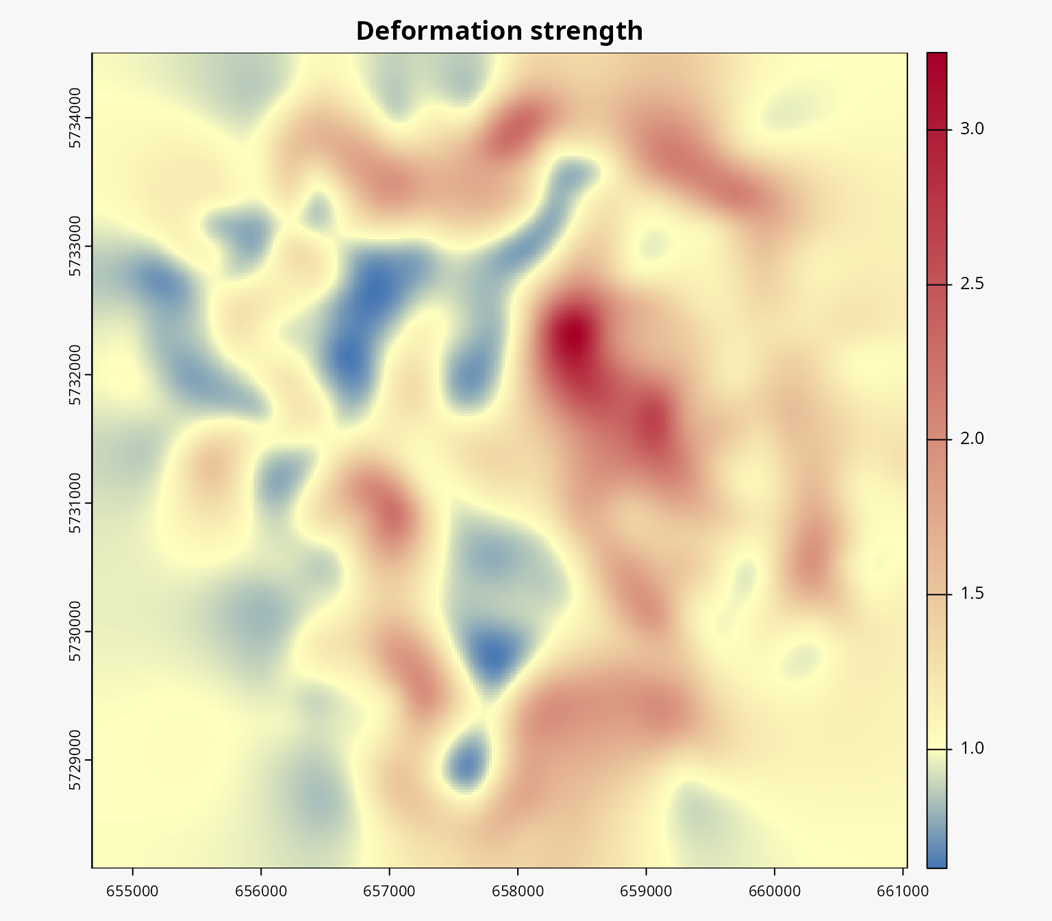
summary(igrid)
#> Summary of the interpolation grid:
#> Number of cells: 900 
#> Precision: 211.693 (α = 2) 
#> Deformation strength: 1.2912 
#> Mean absolute error: 64.47526 
#> RMSE (interp - image): 81.72795 
#> RMSE x (interp - image): 51.80675 
#> RMSE y (interp - image): 63.21011 
#> RMSE (interp - source): 598.5697 
#> RMSE x (interp - source): 469.7113 
#> RMSE y (interp - source): 371.0216 
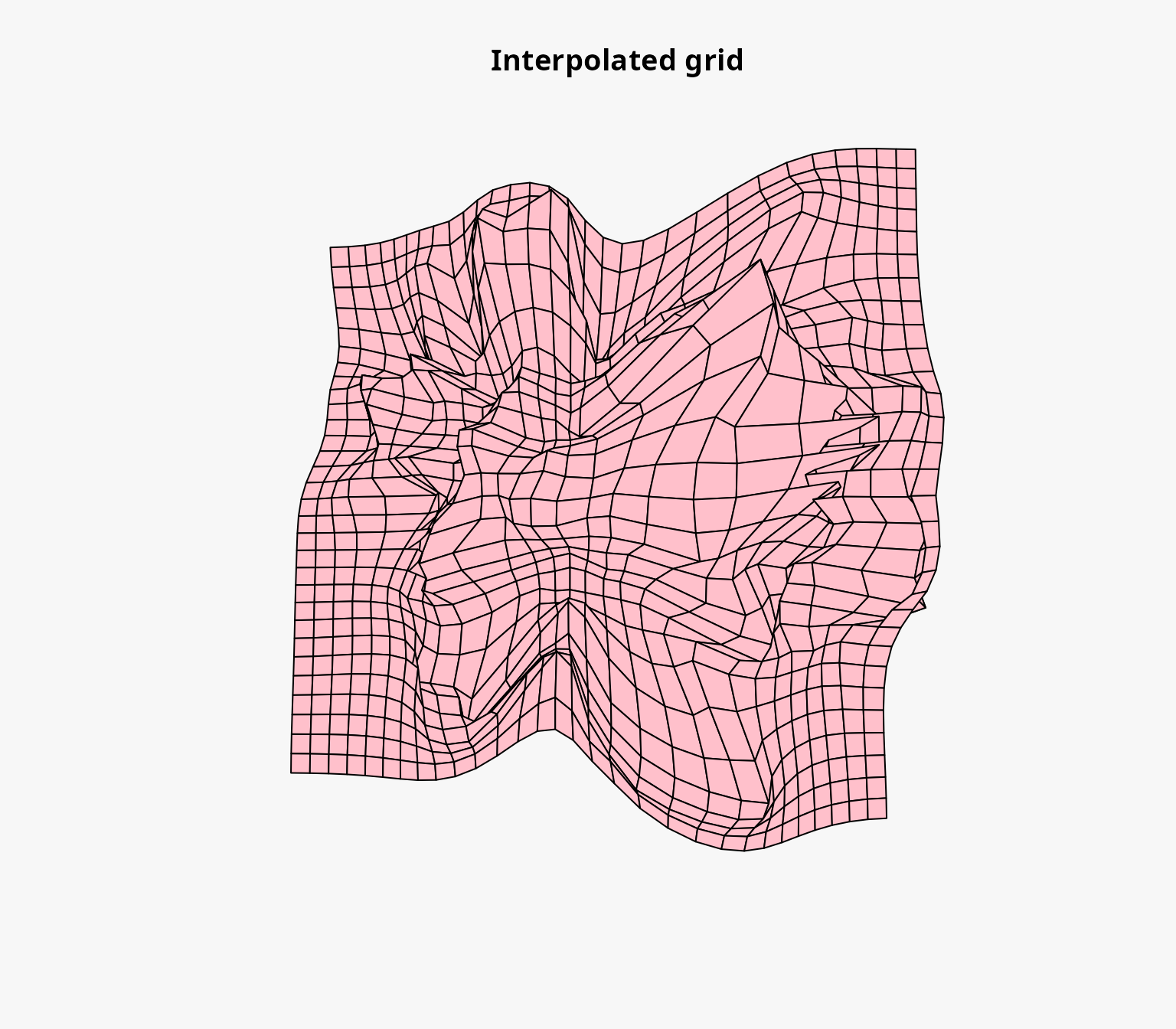
#> R squared: 0.9985654

We can also plot the interpolation grid to visualize the source grid, the interpolated grid, the distance between the image points and the interpolated points, and the strength of the deformation.

plot(igrid)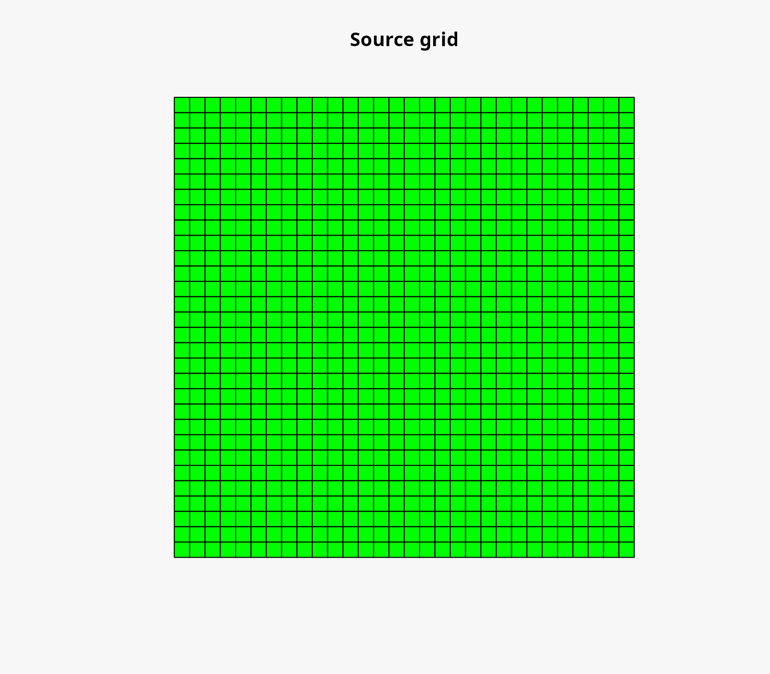

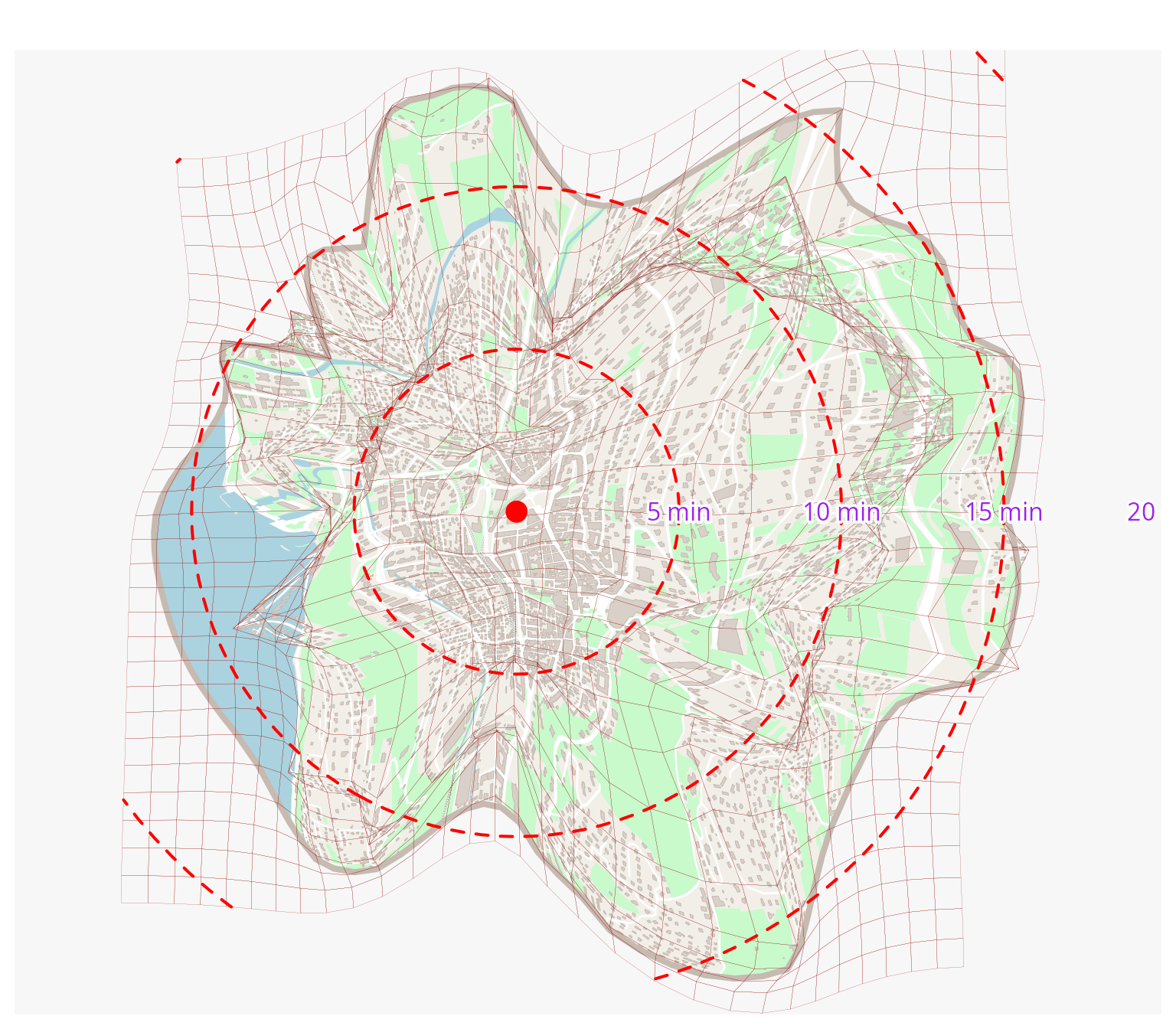
Deforming the background layers

Since we have multiple layers to deform, we can use the dc_interpolate_parallel function to deform all the layers at once:

deformed <- dc_interpolate_parallel(igrid, res)

Mapping the result

mf_map(deformed$circle, col = "#f2efe9", border = NA, add = FALSE)
mf_map(deformed$green, col = "#c8facc", border = "#c8facc", lwd = .5, add = TRUE)
mf_map(deformed$water, col = "#aad3df", border = "#aad3df", lwd = .5, add = TRUE)
mf_map(deformed$railway, col = "grey50", lty = 2, lwd = .2, add = TRUE)
mf_map(deformed$road, col = "white", border = "white", lwd = .5, add = TRUE)
mf_map(deformed$street, col = "white", border = "white", lwd = .5, add = TRUE)
mf_map(deformed$building, col = "#d9d0c9", border = "#c6bab1", lwd = .5, add = TRUE)
mf_map(deformed$circle, col = NA, border = "#c6bab1", lwd = 4, add = TRUE)
mf_map(igrid$interpolated_grid, col = NA, border = "#940000", lwd = .1, add = TRUE)
mf_map(start, pch = 16, col = "red", cex = 2, add = TRUE)
mf_map(sf::st_intersection(circles, sf::st_union(sf::st_buffer(igrid$interpolated_grid, 0))), col = "red", lty = 2, lwd = 2, add = TRUE)

for (i in 1:4) {
  mapsf:::shadowtext(
    sf::st_bbox(circles$geometry[i])$xmax,
    start$geometry[[1]][2],
    paste(i * 5, "min"),
    col = "purple",
    bg = "white",
    r = 0.15
  )
}

If needed, we can add the various points (or a sample of them) and their corresponding travel times to see that the deformation has been correctly applied:

mvd_pts <- igrid$interpolated_points
mvd_pts$durations <- c(0, points$durations)

mf_map(deformed$circle, col = "#f2efe9", border = NA, add = FALSE)
mf_map(deformed$green, col = "#c8facc", border = "#c8facc", lwd = .5, add = TRUE)
mf_map(deformed$water, col = "#aad3df", border = "#aad3df", lwd = .5, add = TRUE)
mf_map(deformed$railway, col = "grey50", lty = 2, lwd = .2, add = TRUE)
mf_map(deformed$road, col = "white", border = "white", lwd = .5, add = TRUE)
mf_map(deformed$street, col = "white", border = "white", lwd = .5, add = TRUE)
mf_map(deformed$building, col = "#d9d0c9", border = "#c6bab1", lwd = .5, add = TRUE)
mf_map(deformed$circle, col = NA, border = "#c6bab1", lwd = 4, add = TRUE)
mf_map(igrid$interpolated_grid, col = NA, border = "#940000", lwd = .1, add = TRUE)
mf_map(start, pch = 16, col = "red", cex = 2, add = TRUE)
mf_map(sf::st_intersection(circles, sf::st_union(sf::st_buffer(igrid$interpolated_grid, 0))), col = "red", lty = 2, lwd = 2, add = TRUE)

for (i in 1:4) {
  mapsf:::shadowtext(
    sf::st_bbox(circles$geometry[i])$xmax,
    start$geometry[[1]][2],
    paste(i * 5, "min"),
    col = "purple",
    bg = "white",
    r = 0.15
  )
}

mf_map(mvd_pts, add = TRUE, col = "blue")
mf_label(mvd_pts, var = "durations", col = "black", halo = TRUE, overlap = TRUE)

Conclusion

Distance cartograms are both a way of analyzing space and a way of representing it. In the case of unipolar cartograms, as proposed here, reading is generally fairly straightforward, making it easy to highlight portions of the territory that are difficult (or at least more difficult than the average) to reach for example.

Matthieu Viry

2025-02-03