Hello geovizr

The geovizr package is a (partial) R interface to the geoviz JavaScript library. It allows users to create vector-based, interactive, and zoomable thematic maps.

The geovizr package is an R wrapper around the geoviz JavaScript library via a htmlwidget. Its development follows the evolution of the library. The parameter names are the same. You can therefore refer to the JavaScript geoviz documentation here.
Since it’s based on d3.js, the philosophy behind this package is completely different as other R mapping packages. Map parameters use svg attributes rather than the usual R parameters. Thus, strokeWidth is used rather than lwd, fill rather than col, stroke rather than border, etc.
geovizr is not designed to handle voluminous datasets. It is suitable for light, generalized basemaps.
geovizr is designed to work with geographic data in wgs84 (not projected). Geometries are then projected on the fly using the create() function. Unlike other R packages based on sf, the projections used come from the d3.js ecosystem (d3-geo, d3-geo-projection & d3-geo-polygon).
Maps generated by geovizr are zoomable. Two types of zoom are available. The classic type (pan and zoom) and the “versor” type for creating interactive globes.
Maps created with geovizr are interactive. It is therefore possible to create tooltips to access information contained in geographic objects.
Many different types of maps are available. The types can be combined with each other and are highly customizable.

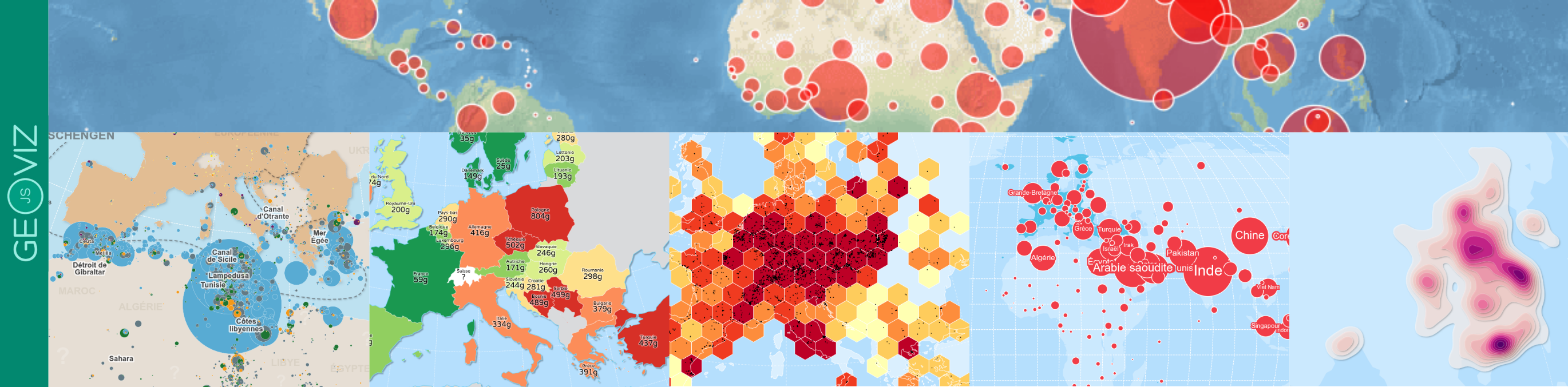
Here an example of a map designed with the package:

Installation

You can install the released version of geovizr from CRAN with:

install.packages("geovizr")

Alternatively, you can install the development version of geovizr from r-universe with:

install.packages("geovizr", repos = c("https://riatelab.r-universe.dev", "https://cloud.r-project.org"))

then

library(geovizr)

Syntax

There are several steps involved in creating a map with geovizr.

1 - First, create the map container using the create() function. This is where you define the projection, margins, background color, etc. - in short, all the general parameters of the map.

2 The next step is to progressively add layers. A set of dedicated functions is available for this purpose. For instance, viz_path() adds a spatial dataframe, viz_graticule() draws latitude and longitude lines, viz_header() inserts a title, and viz_footer() adds a source note. All available functions are documented in the Reference section.

3 - Then, the render() function displays the map

The various functions can be chained together with a pipe (|>).

Now, let’s build a world map.

# Data Loading
library(sf)

world <- st_read(
  system.file("gpkg/world.gpkg", package = "geovizr"),
  quiet = TRUE
)

cities <- st_read(
  system.file("gpkg/cities.gpkg", package = "geovizr"),
  quiet = TRUE
)

⚠️ The geometries must be in latitude and longitude coordinates, not projected. Use WGS84.

viz_create() |>
  viz_outline() |>
  viz_graticule() |>
  viz_path(data = world) |>
  viz_path(data = cities) |>
  viz_header(text = "Hello World") |>
  viz_render()

Styling

As you can see, the name of the parameters don’t look like classical R parameters. Since it’s based on d3.js, map parameters use svg attributes rather than the usual R parameters. Thus, strokeWidth is used rather than lwd, fill rather than col, stroke rather than border, etc.

All layers have default parameters, but you can modify them. Here is a list of parameters you can use on most layers:

fill: Sets the fill color of the element. Can be a fixed color (e.g., “steelblue”) or a function mapping a data variable to colors.
stroke: Sets the color of the element’s outline (border). Example: “#000” for black.
strokeWidth: Width of the outline in pixels. Controls how thick the border appears.
opacity: Overall opacity of the element, from 0 (fully transparent) to 1 (fully opaque).
fillOpacity: Opacity of the fill only, separate from the stroke.
strokeOpacity: Opacity of the stroke only.
strokeDasharray: Defines a dash pattern for the stroke. Example: “5,5” creates dashed lines of 5px segments with 5px gaps.
strokeLinecap: Defines the shape of the ends of lines. Values: “butt”, “round”, “square”.
strokeLinejoin: Defines the shape of joints between connected lines. Values: “miter”, “round”, “bevel”.

⚠️ Be careful: pay attention to uppercase and lowercase letters.

Let’s take the previous map and customize it to our liking.

viz_create() |>
  viz_outline(fill = "#38896F", fillOpacity = 0.3) |>
  viz_graticule(stroke = "white", step = 20) |>
  viz_path(
    data = world, fill = "white",
    stroke = "none", fillOpacity = 0.3
  ) |>
  viz_path(
    data = cities, pointRadius = 2,
    stroke = "none", fill = "#38896F"
  ) |>
  viz_header(
    text = "Hello World", fill = "white",
    background_fill = "#38896F"
  ) |>
  viz_render()

Positioning of elements

To position symbols or text on the map, we most often use the coordinates from a spatial dataframe. However, it is also possible to place specific elements at precise coordinates. For this, two coordinate systems coexist in geovizr:

Geographical coordinates

By specifying coords = "geo", you can position an element at precise geographic coordinates. The object is then linked to the map and stays in the correct location according to the zoom level.

# A simple map
mumbai <- c(72.88, 19.07)
viz_create(zoomable = T) |>
  viz_path(data = world, fill = "#CCC", stroke = "none", fillOpacity = 0.3) |>
  viz_circle(pos = mumbai, coords = "geo", fill = "#38896F", r = 10) |>
  viz_render()

SVG coordinates

By specifying coords = "svg", you can also position an element statically directly on the map plane. This is very useful for decorative elements, such as the legend or text labels.

⚠️ The origin of the coordinate system used to express coordinates in an SVG document is located at the top left.

# A simple map
viz_create(zoomable = T) |>
  viz_path(data = world, fill = "#CCC", stroke = "none", fillOpacity = 0.3) |>
  viz_circle(pos = c(300, 100), coords = "svg", fill = "#38896F", r = 10) |>
  viz_render()

Symbology

Specialized functions are available for representing statistical data, whether qualitative or quantitative. For example:

viz_choro(): for relative quantitative data
viz_prop(): for absolute quantitative data
viz_typo(): for qualitative data

These functions take two main parameters: data for the base map and var for the variable to be mapped. Additional parameters allow for fine customization of both the map and its legend.

Here is a simple example of a proportional symbol map

viz_create() |>
  viz_path(datum = world, fill = "#CCC") |>
  viz_prop(data = world, var = "pop", fill = "#38896F") |>
  viz_render()

A choropleth map

viz_create() |>
  viz_choro(data = world, var = "gdppc", fill = "#38896F") |>
  viz_render()

And a typology

viz_create() |>
  viz_typo(data = world, var = "region") |>
  viz_render()

For more details, see the “symbology” page.

Nicolas Lambert

2026-06-10

Installation

Syntax

Styling

Positioning of elements

Symbology