Choropleth Layer

Plot a choropleth layer.

choroLayer(
  x,
  spdf,
  df,
  spdfid = NULL,
  dfid = NULL,
  var,
  breaks = NULL,
  method = "quantile",
  nclass = NULL,
  col = NULL,
  border = "grey20",
  lwd = 1,
  colNA = "white",
  legend.pos = "bottomleft",
  legend.title.txt = var,
  legend.title.cex = 0.8,
  legend.values.cex = 0.6,
  legend.values.rnd = 0,
  legend.nodata = "no data",
  legend.frame = FALSE,
  legend.border = "black",
  legend.horiz = FALSE,
  add = FALSE
)

Arguments

x: an sf object, a simple feature collection. If x is used then spdf, df, spdfid and dfid are not.
spdf: a SpatialPolygonsDataFrame.
df: a data frame that contains the values to plot. If df is missing spdf@data is used instead.
spdfid: name of the identifier variable in spdf, default to the first column of the spdf data frame. (optional)
dfid: name of the identifier variable in df, default to the first column of df. (optional)
var: name of the numeric variable to plot.
breaks: break values in sorted order to indicate the intervals for assigning the colors. Note that if there are nlevel colors (classes) there should be (nlevel+1) break values (see Details).
method: a classification method; one of "sd", "equal", "quantile", "fisher-jenks","q6", "geom", "arith", "em" or "msd" (see getBreaks).
nclass: a targeted number of classes. If null, the number of class is automatically defined (see Details).
col: a vector of colors. Note that if breaks is specified there must be one less colors specified than the number of break.
border: color of the polygons borders.
lwd: borders width.
colNA: no data color.
legend.pos: position of the legend, one of "topleft", "top", "topright", "right", "bottomright", "bottom", "bottomleft", "left" or a vector of two coordinates in map units (c(x, y)). If legend.pos is "n" then the legend is not plotted.
legend.title.txt: title of the legend.
legend.title.cex: size of the legend title.
legend.values.cex: size of the values in the legend.
legend.values.rnd: number of decimal places of the values in the legend.
legend.nodata: no data label.
legend.frame: whether to add a frame to the legend (TRUE) or not (FALSE).
legend.border: color of boxes borders in the legend.
legend.horiz: whether to display the legend horizontally (TRUE) or not (FALSE).
add: whether to add the layer to an existing plot (TRUE) or not (FALSE).

Details

The optimum number of class depends on the number of geographical objects. If nclass is not defined, an automatic method inspired by Sturges (1926) is used : nclass = 1+3.3*log10(N), where nclass is the number of class and N is the variable length.

If breaks is used then nclass and method are not.

If breaks is defined as c(2, 5, 10, 15, 20) intervals will be: [2 - 5[, [5 - 10[, [10 - 15[, [15 - 20].

References

Herbert A. Sturges, « The Choice of a Class Interval », Journal of the American Statistical Association, vol. 21, n° 153, mars 1926, p. 65-66.

Examples

library(sf)
mtq <- st_read(system.file("gpkg/mtq.gpkg", package="cartography"))
#> Reading layer `mtq' from data source 
#>   `/tmp/RtmpmpfIrO/temp_libpath18ee15f22a9e/cartography/gpkg/mtq.gpkg' 
#>   using driver `GPKG'
#> Simple feature collection with 34 features and 7 fields
#> Geometry type: MULTIPOLYGON
#> Dimension:     XY
#> Bounding box:  xmin: 690574 ymin: 1592536 xmax: 735940.2 ymax: 1645660
#> Projected CRS: WGS 84 / UTM zone 20N
# Population density
mtq$POPDENS <- 1e6 * mtq$POP / st_area(x = mtq)

# Default
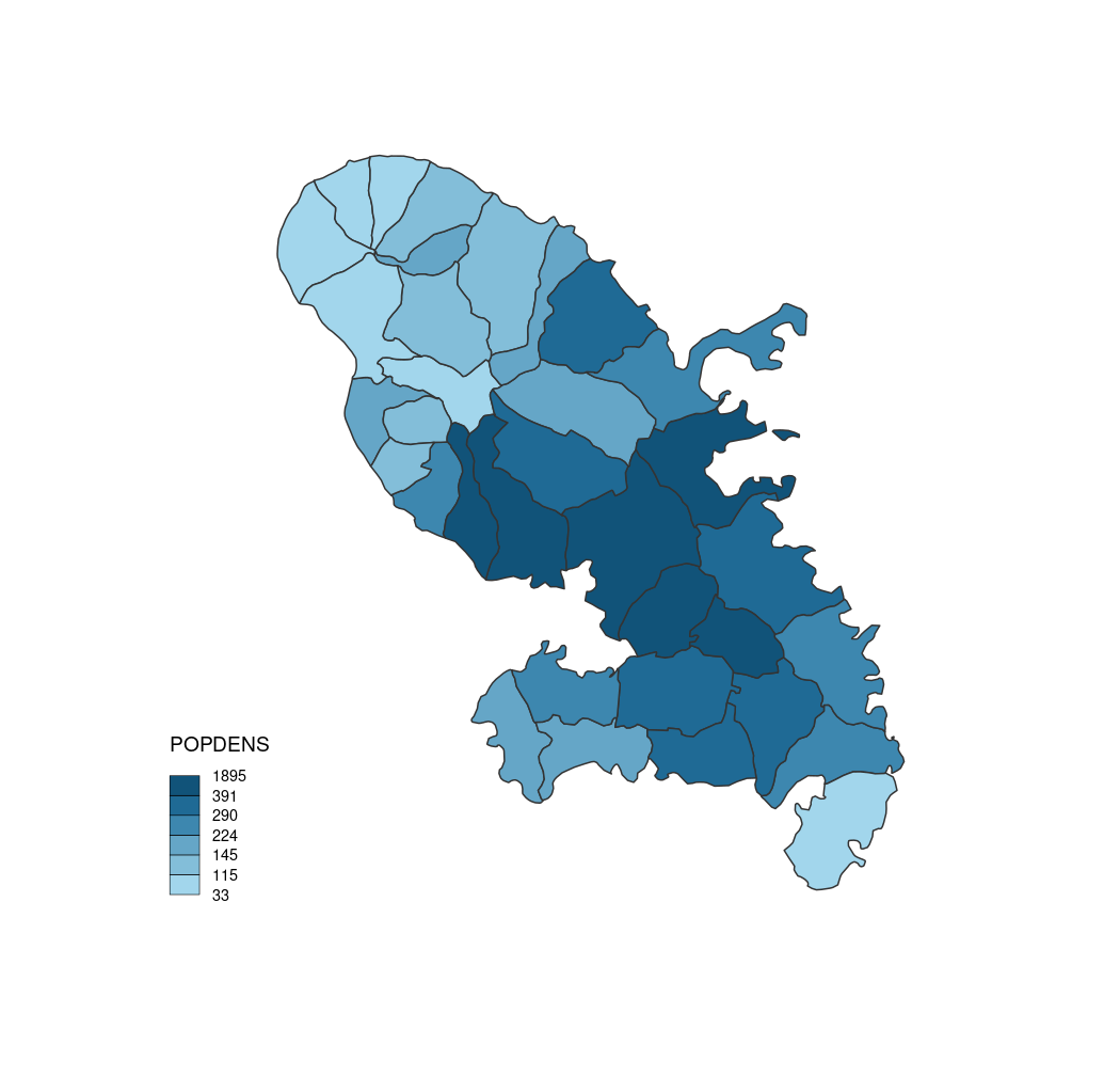
choroLayer(x = mtq, var = "POPDENS")


# With parameters 
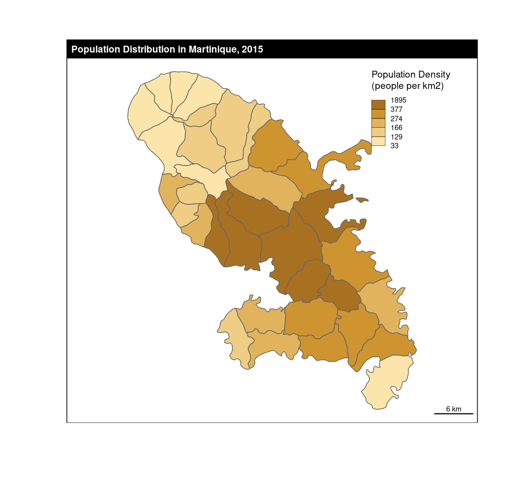
choroLayer(x = mtq, var = "POPDENS",
           method = "quantile", nclass = 5,
           col = carto.pal(pal1 = "sand.pal", n1 = 5),
           border = "grey40",
           legend.pos = "topright", legend.values.rnd = 0,
           legend.title.txt = "Population Density\n(people per km2)")

# Layout
layoutLayer(title = "Population Distribution in Martinique, 2015")

Arguments

Details

References

See also

Examples