cartography
Timothée Giraud, Nicolas Lambert
2023-01-18
Source:vignettes/cartography.Rmd
cartography.RmdIntroduction
The aim of cartography is to obtain thematic maps with
the visual quality of those build with a classical mapping or GIS
software.
Users of the package could belong to one of two categories: cartographers willing to use R or R users willing to create maps. Therefore, its functions have to be intuitive to cartographers and ensure compatibility with common R workflows.
cartography uses sf or sp objects
to produce base graphics. As most of the internals of the
package relies on sf functionalities, the preferred format
for spatial objects is sf.
Features
cartography’s functions can be classified in the
following categories :
-
Symbology
Each function focuses on a single cartographic representation (e.g. proportional symbols or choropleth representation) and displays it on a georeferenced plot. This solution allows to consider each representation as a layer and to overlay multiple representations on a same map.
Each function has two main arguments that are:-
x, a spatial object (preferably ansfobject),
-
var, the name of a variable to map.
spobjects are handled through thespdfargument if the variable is contained within theSpatial*DataFrameand throughspdf,spdfid,df,dfidif the variable is in a separatedata.framethat needs to be joined to theSpatial*DataFrame.Many parameters are available to fine tune the cartographic representations. These parameters are the common ones found in GIS and automatic cartography tools (e.g. classification and color palettes used in choropleth maps, symbols sizes used in proportional symbols maps…).
-
Transformations
A set of functions is dedicated to the creation or transformation of spatial objects (e.g. borders extraction, grid or links creation). These functions are provided to ease the creation of some more advanced maps that usually need geo-processing.Map Layout
Along with the cartographic functions, some other functions are dedicated to layout design (e.g. customizable scale bar, north arrow, title, sources or author information…).Color Palettes
16 original color palettes are shipped within the package. Those palettes can be customized and combined.Legends
Legends are displayed by default along cartographic layers but more parameters are available throughlegend*()functions.Classification
getBreaks()give access to most of the classification methods used for data binning.
Examples of thematic maps
Proportional Symbols
propSymbolsLayer() displays symbols with areas
proportional to a quantitative variable (stocks). Several symbols are
available (circles, squares, bars). The inches argument is
used to customize the symbols sizes.
library(sf)
library(cartography)
# path to the geopackage file embedded in cartography
path_to_gpkg <- system.file("gpkg/mtq.gpkg", package="cartography")
# import to an sf object
mtq <- st_read(dsn = path_to_gpkg, quiet = TRUE)
# plot municipalities (only borders are plotted)
plot(st_geometry(mtq), col = "grey80", border = "grey")
# plot population
propSymbolsLayer(
  x = mtq,
  var = "POP",
  inches = 0.25,
  col = "brown4",
  legend.pos = "topright",
  legend.title.txt = "Total population"
)
# layout
layoutLayer(title = "Population Distribution in Martinique",
            sources = "Sources: Insee and IGN, 2018",
            author = paste0("cartography ", packageVersion("cartography")),
            frame = FALSE, north = FALSE, tabtitle = TRUE)
# north arrow
north(pos = "topleft")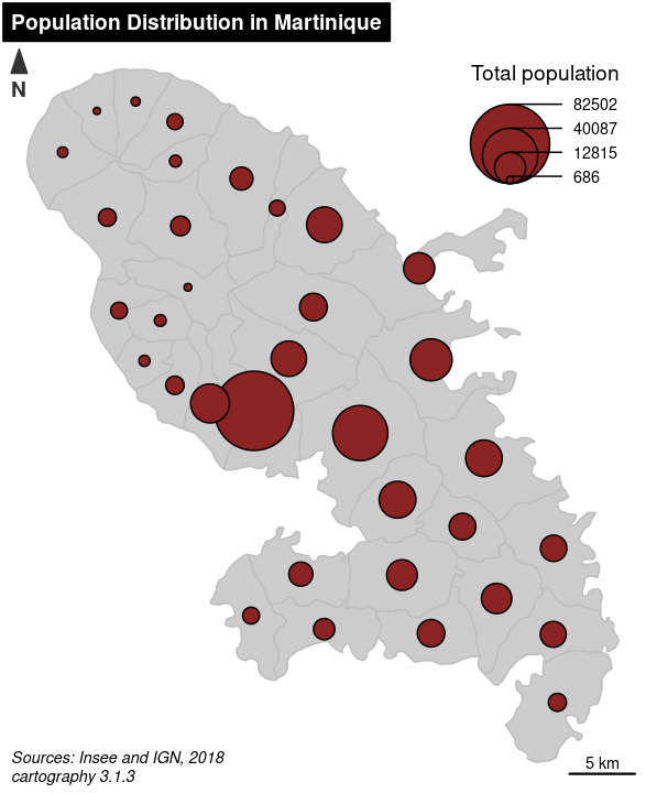
Choropleth Map
In choropleth maps, areas are shaded according to the variation of a quantitative variable. They are used to represent ratios or indices.
choroLayer() displays choropleth maps . Arguments
nclass, method and breaks allow
to customize the variable classification. getBreaks() allow
to classify outside of the function itself. Colors palettes are defined
with col and a set of colors can be created with
carto.pal() (see also display.carto.all()).
library(sf)
library(cartography)
# path to the geopackage file embedded in cartography
path_to_gpkg <- system.file("gpkg/mtq.gpkg", package="cartography")
# import to an sf object
mtq <- st_read(dsn = path_to_gpkg, quiet = TRUE)
# population density (inhab./km2) using sf::st_area()
mtq$POPDENS <- 1e6 * mtq$POP / st_area(mtq)
# plot municipalities (only the backgroung color is plotted)
plot(st_geometry(mtq), col = NA, border = NA, bg = "#aadaff")
# plot population density
choroLayer(
  x = mtq,
  var = "POPDENS",
  method = "geom",
  nclass=5,
  col = carto.pal(pal1 = "sand.pal", n1 = 5),
  border = "white",
  lwd = 0.5,
  legend.pos = "topright",
  legend.title.txt = "Population Density\n(people per km2)",
  add = TRUE
)
# layout
layoutLayer(title = "Population Distribution in Martinique",
            sources = "Sources: Insee and IGN, 2018",
            author = paste0("cartography ", packageVersion("cartography")),
            frame = FALSE, north = FALSE, tabtitle = TRUE, theme= "sand.pal")
# north arrow
north(pos = "topleft")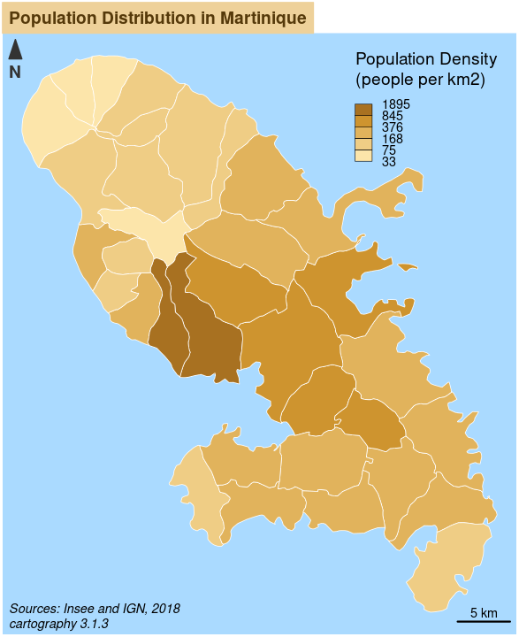
Colored Pencil and Typologies Map
getPencilLayer() transforms POLYGONS or MULTIPOLYGONS in
MULTILINESTRINGS. This function creates a layer that mimicks a pencil
hand-drawing.
typoLayer() displays a typology map of a qualitative
variable. legend.values.order is used to set the modalities
order in the legend.
library(sf)
library(cartography)
# path to the geopackage file embedded in cartography
path_to_gpkg <- system.file("gpkg/mtq.gpkg", package="cartography")
# import to an sf object
mtq <- st_read(dsn = path_to_gpkg, quiet = TRUE)
# transform municipality multipolygons to (multi)linestrings
mtq_pencil <- getPencilLayer(
  x = mtq,
  size = 400,
  lefthanded = F
)
# plot municipalities (only the backgroung color is plotted)
plot(st_geometry(mtq), col = "white", border = NA, bg = "lightblue1")
# plot administrative status
typoLayer(
  x = mtq_pencil,
  var="STATUS",
  col = c("aquamarine4", "yellow3","wheat"),
  lwd = .7,
  legend.values.order = c("Prefecture",
                          "Sub-prefecture",
                          "Simple municipality"),
  legend.pos = "topright",
  legend.title.txt = "",
  add = TRUE
)
#  plot municipalities
plot(st_geometry(mtq), lwd = 0.5, border = "grey20", add = TRUE, lty = 3)
# labels for a few  municipalities
labelLayer(x = mtq[mtq$STATUS != "Simple municipality",], txt = "LIBGEO",
           cex = 0.9, halo = TRUE, r = 0.15)
# title, source, author
layoutLayer(title = "Administrative Status",
            sources = "Sources: Insee and IGN, 2018",
            author = paste0("cartography ", packageVersion("cartography")),
            north = FALSE, tabtitle = TRUE, postitle = "right",
            col = "white", coltitle = "black")
# north arrow
north(pos = "topleft")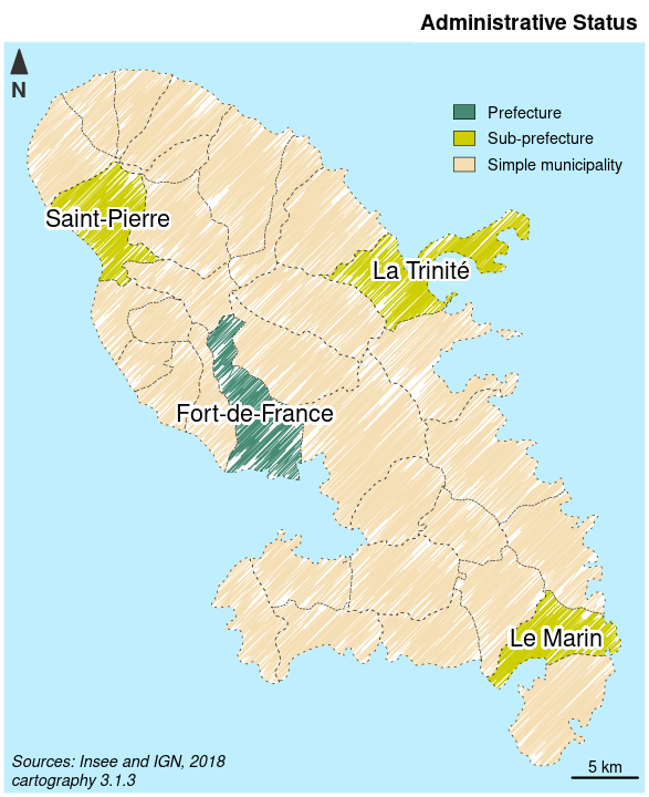
Proportional Symbols and Choropleth Map
propSymbolsChoroLayer() creates a map of symbols that
are proportional to values of a first variable and colored to reflect
the classification of a second variable. A combination of
propSymbolsLayer() and choroLayer() arguments
is used.
library(sf)
library(cartography)
# path to the geopackage file embedded in cartography
path_to_gpkg <- system.file("gpkg/mtq.gpkg", package="cartography")
# import to an sf object
mtq <- st_read(dsn = path_to_gpkg, quiet = TRUE)
# Plot the municipalities
plot(st_geometry(mtq), col="darkseagreen3", border="darkseagreen4",
     bg = "lightblue1", lwd = 0.5)
# Plot symbols with choropleth coloration
propSymbolsChoroLayer(
  x = mtq,
  var = "POP",
  border = "grey50",
  lwd = 1,
  legend.var.pos = "topright",
  legend.var.title.txt = "Population",
  var2 = "MED",
  method = "equal",
  nclass = 4,
  col = carto.pal(pal1 = "sand.pal", n1 = 4),
  legend.var2.values.rnd = -2,
  legend.var2.pos = "left",
  legend.var2.title.txt = "Median\nIncome\n(in euros)"
)
# layout
layoutLayer(title="Population & Wealth in Martinique, 2015",
            author = "cartography 2.1.3",
            sources = "Sources: Insee and IGN, 2018",
            scale = 5, tabtitle = TRUE, frame = FALSE)
# north arrow
north(pos = "topleft")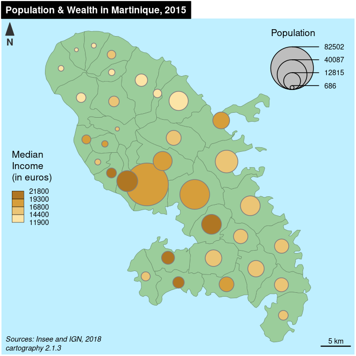
Proportional Symbols and Typology Map
propSymbolsTypoLayer() creates a map of symbols that are
proportional to values of a first variable and colored to reflect the
modalities of a second qualitatice variable. A combination of
propSymbolsLayer() and typoLayer() arguments
is used.
library(sf)
library(cartography)
# path to the geopackage file embedded in cartography
path_to_gpkg <- system.file("gpkg/mtq.gpkg", package="cartography")
# import to an sf object
mtq <- st_read(dsn = path_to_gpkg, quiet = TRUE)
# Plot the municipalities
plot(st_geometry(mtq), col="#f2efe9", border="#b38e43", bg = "#aad3df",
     lwd = 0.5)
# Plot symbols with choropleth coloration
propSymbolsTypoLayer(
  x = mtq,
  var = "POP",
  inches = 0.5,
  symbols = "square",
  border = "white",
  lwd = .5,
  legend.var.pos = "topright",
  legend.var.title.txt = "Population",
  var2 = "STATUS",
  legend.var2.values.order = c("Prefecture", "Sub-prefecture",
                               "Simple municipality"),
  col = carto.pal(pal1 = "multi.pal", n1 = 3),
  legend.var2.pos = c(692000, 1607000),
  legend.var2.title.txt = "Administrative\nStatus"
)
# layout
layoutLayer(title="Population Distribution in Martinique",
            author = "cartography 2.1.3",
            sources = "Sources: Insee and IGN, 2018",
            scale = 5, tabtitle = TRUE, frame = FALSE)
# north arrow
north(pos = "topleft")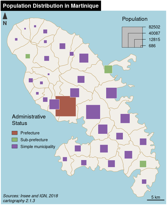
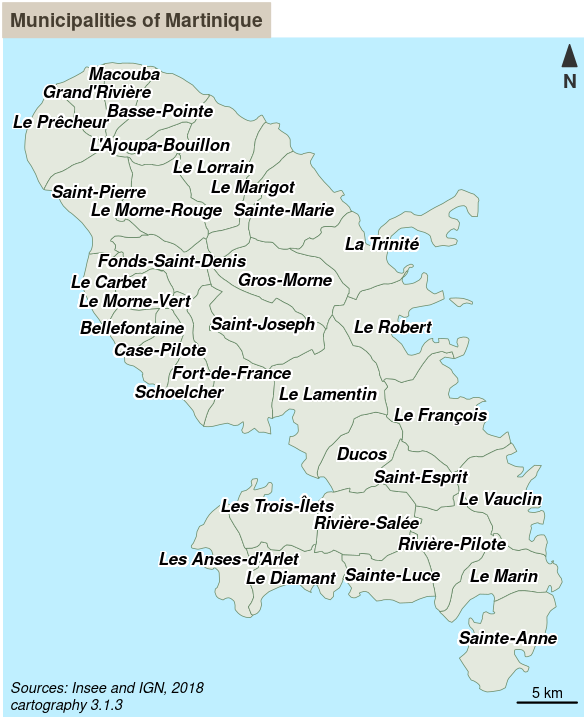
Label Map
labelLayer() is dedicated to the display of labels on a
map. The overlap = FALSE argument displays non overlapping
labels.
library(sf)
library(cartography)
# path to the geopackage file embedded in cartography
path_to_gpkg <- system.file("gpkg/mtq.gpkg", package="cartography")
# import to an sf object
mtq <- st_read(dsn = path_to_gpkg, quiet = TRUE)
# plot municipalities
plot(st_geometry(mtq), col = "#e4e9de", border = "darkseagreen4",
     bg = "lightblue1", lwd = 0.5)
# plot labels
labelLayer(
  x = mtq,
  txt = "LIBGEO",
  col= "black",
  cex = 0.7,
  font = 4,
  halo = TRUE,
  bg = "white",
  r = 0.1,
  overlap = FALSE,
  show.lines = FALSE
)
# map layout
layoutLayer(
  title = "Municipalities of Martinique",
  sources = "Sources: Insee and IGN, 2018",
  author = paste0("cartography ", packageVersion("cartography")),
  frame = FALSE,
  north = TRUE,
  tabtitle = TRUE,
  theme = "taupe.pal"
) 
Links Map
getLinkLayer() creates a link layer from an
sf object and a link data.frame (long
format).gradLinkTypoLayer() displays graduated and colored
links.
library(sf)
library(cartography)
# path to the geopackage file embedded in cartography
path_to_gpkg <- system.file("gpkg/mtq.gpkg", package="cartography")
# import to an sf object
mtq <- st_read(dsn = path_to_gpkg, quiet = TRUE)
# path to the csv file embedded in cartography
path_to_csv <- system.file("csv/mob.csv", package="cartography")
# import to a data.frame
mob <- read.csv(path_to_csv)
# select workplaces with administrative status = Prefecture or Sub-prefecture
mob <- mob[mob$sj != "Simple municipality",]
# create an sf object of links
mtq_mob <- getLinkLayer(
  x = mtq,
  xid = "INSEE_COM",
  df = mob,
  dfid = c("i","j")
)
# set figure background color
par(bg="grey25")
# plot municipalities
plot(st_geometry(mtq), col = "grey13", border = "grey25",
     bg = "grey25", lwd = 0.5)
# plot graduated links
gradLinkTypoLayer(
  x = mtq_mob,
  xid = c("i", "j"),
  df = mob,
  dfid = c("i","j"),
  var = "fij",
  breaks = c( 100,  500, 1200, 2500, 4679.0),
  lwd = c(1,4,8,16),
  legend.var.pos = "left",
  legend.var.title.txt = "Nb. of\nCommuters",
  var2 = "sj",
  col = c("grey85", "red4"),
  legend.var2.title.txt = "Workplace",
  legend.var2.pos = "topright"
)
# map layout
layoutLayer(title = "Commuting to Prefectures in Martinique",
            sources = "Sources: Insee and IGN, 2018",
            author = paste0("cartography ", packageVersion("cartography")),
            frame = FALSE, col = "grey25", coltitle = "white",
            tabtitle = TRUE)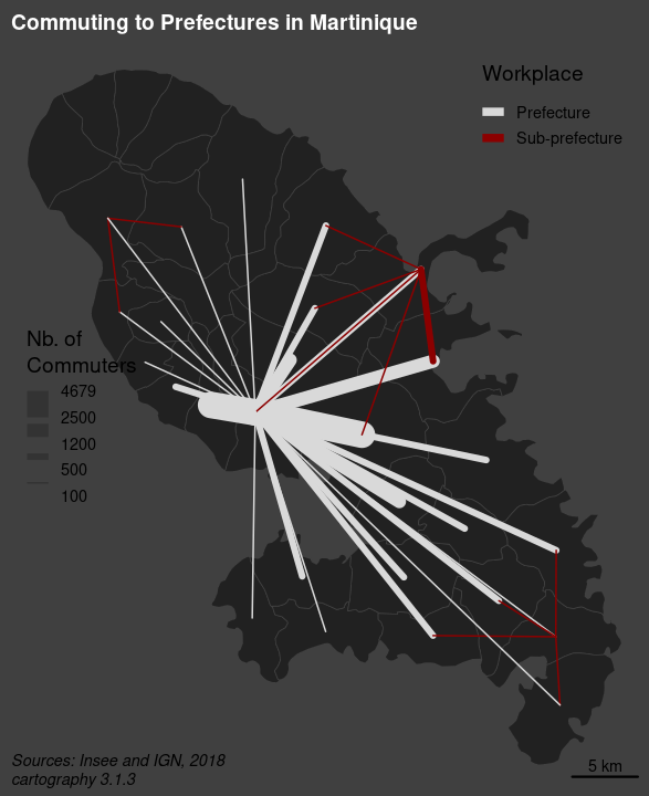
Isopleth Map
smoothLayer() is deprecated. See the package potential
instead.
Isopleth maps are based on the assumption that the phenomenon to be represented has a continuous distribution. These maps use a spatial interaction modeling approach which aims to compute indicators based on stock values weighted by distance. It allows a spatial representation of the phenomenon independent from the initial heterogeneity of the territorial division.
Grid Map
The grid-cell method is an option to overcome the arbitrariness and
irregularity of an administrative division. It highlights the main
trends in the data spatial distribution, splitting the territory in
regular blocks. Statistical values are distributed over a regular grid.
Cell values are classified and then displayed in areas of color. The
principle adopted here is to set each cell’s value with a proportion of
the initial geometrical units it overlay (share of intersected
area).getGridLayer() builds a regular grid (squares or hexagons)
based on a spatial object and computes data that match the grid layer.
choroLayer() is then used to display the grid on a
choropleth map.
library(sf)
library(cartography)
# path to the geopackage file embedded in cartography
path_to_gpkg <- system.file("gpkg/mtq.gpkg", package="cartography")
# import to an sf object
mtq <- st_read(dsn = path_to_gpkg, quiet = TRUE)
# Create a grid layer, cell size area match the median municipality area
mygrid <- getGridLayer(
  x = mtq,
  cellsize = median(as.numeric(st_area(mtq))),
  var = "POP",
  type = "hexagonal"
)
# Compute population density in people per km2
mygrid$POPDENS <- 1e6 * mygrid$POP / mygrid$gridarea
# plot municipalities (only the backgroung color is plotted)
plot(st_geometry(mtq), col = NA, border = NA, bg = "#deffff")
# Plot the population density
choroLayer(x = mygrid, var = "POPDENS", method = "geom", nclass=5,
           col = carto.pal(pal1 = "turquoise.pal", n1 = 5), border = "grey80",
           lwd = 0.5, legend.pos = "bottomleftextra", add = TRUE,
           legend.title.txt = "Population Density\n(people per km2)")
layoutLayer(title = "Population Distribution in Martinique",
            sources = "Sources: Insee and IGN, 2018",
            author = paste0("cartography ", packageVersion("cartography")),
            frame = FALSE, north = FALSE, tabtitle = TRUE,
            theme = "turquoise.pal")
# north arrow
north(pos = "topleft")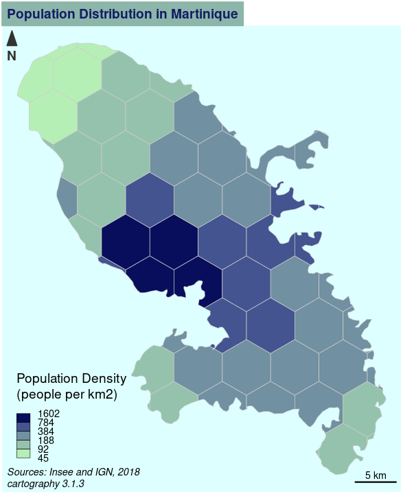
Discontinuities Map
Discontinuities maps are based on the variation of a phenomena
between contiguous units. This kind of representation focuses spatial
breaks. The discontinuity intensity is expressed by the borders’
thickness.getBorders() is used to build a spatial object of borders
between units. Each resulting borders contains the ids of its two
neighboring units. It is possible to complement these borders with
getOuterBorders() to compute borders between non-contiguous
units (e.g. maritime borders). discLayer() computes and
displays discontinuities, lines widths reflect the ratio or the absolute
difference between values of an indicator in two neighboring units.
library(sf)
library(cartography)
# path to the geopackage file embedded in cartography
path_to_gpkg <- system.file("gpkg/mtq.gpkg", package="cartography")
# import to an sf object
mtq <- st_read(dsn = path_to_gpkg, quiet = TRUE)
# Compute the population density (inhab./km2) using sf::st_area()
mtq$POPDENS <- as.numeric(1e6 * mtq$POP / st_area(mtq))
# Get a SpatialLinesDataFrame of countries borders
mtq.contig <- getBorders(mtq)
# plot municipalities (only the backgroung color is plotted)
plot(st_geometry(mtq), col = NA, border = NA, bg = "lightblue1",
     xlim = c(690574, 745940))
# Plot the population density with custom breaks
choroLayer(x = mtq, var = "MED",
           breaks = c(min(mtq$MED), seq(13000, 21000, 2000), max(mtq$MED)),
           col = carto.pal("green.pal", 6),border = "white", lwd = 0.5,
           legend.pos = "topright", legend.title.txt = "Median Income\n(euros)",
           add = TRUE)
# Plot discontinuities
discLayer(
  x = mtq.contig,
  df = mtq,
  var = "MED",
  type = "rel",
  method = "geom",
  nclass = 3,
  threshold = 0.4,
  sizemin = 0.7,
  sizemax = 6,
  col = "red4",
  legend.values.rnd = 1,
  legend.title.txt = "Relative\nDiscontinuities",
  legend.pos = "right",
  add = TRUE
)
# Layout
layoutLayer(title = "Wealth Disparities in Martinique, 2015",
            author =  paste0("cartography ", packageVersion("cartography")),
            sources = "Sources: Insee and IGN, 2018",
            frame = FALSE, scale = 5, tabtitle = TRUE,theme = "grey.pal")
# north arrow
north(pos = "topleft")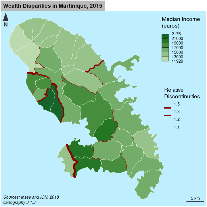
Mapping sp Objects
SpatialPointsDataFrame and
SpatialPolygonsDataFrame (from sp) are handled
through the spdf argument if the variable is contained
within the Spatial*DataFrame and through spdf,
spdfid, df, dfid if the variable
is in a separate data.frame that needs to be joined to the
Spatial*DataFrame.
library(sp)
library(cartography)
data("nuts2006")
# Plot a layer with the extent of the EU28 countries with only a background color
plot(nuts0.spdf, border = NA, col = NA, bg = "#A6CAE0")
# Plot non european space
plot(world.spdf, col  = "#E3DEBF", border = NA, add = TRUE)
# Plot Nuts2 regions
plot(nuts0.spdf, col = "grey60",border = "white", lwd = 0.4, add = TRUE)
# plot the countries population
propSymbolsLayer(
  spdf = nuts0.spdf,
  df = nuts0.df,
  spdfid = "id",
  dfid = "id",
  var = "pop2008",
  legend.pos = "topright",
  col = "red4",
  border = "white",
  legend.title.txt = "Population"
)
# layout
layoutLayer(title = "Population in Europe, 2008",
            sources = "Data: Eurostat, 2008",
            author =  paste0("cartography ", packageVersion("cartography")),
            scale = 500, frame = TRUE, col = "#688994")
# north arrow
north("topleft")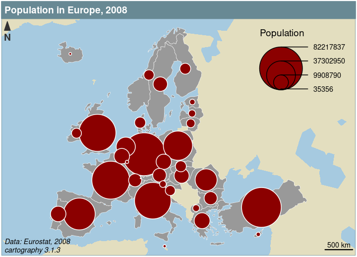
Datasets
Several datasets are embedded in the package:
- A GeoPackage of Martinique
municipalities can be imported via the
st_read()function of thesfpackage.- Sources: Base comparateur de territoires (upload date: 2018-09-25) & ADMIN EXPRESS-COG (2018 edition).
- Citation: Insee and IGN, 2018
- Fields:
- INSEE_COM: Municipality identifier
- STATUS: Municipality administrative status
- LIBGEO: Municipality name
- POP: Total population, 2015
- MED: Median disposable income adjusted per equivalent household member, in euros, 2015
- CHOM: Unemployed population, 2015
- ACT: Active population, 2015
- A csv file of professional mobility flows between Martinique
municipalities.
- Sources: Flux de mobilité - déplacements domicile-lieu de travail (upload date: 2018-08-01)
- Citation: Insee, 2018
- Fields:
- i: Municipality of residence identifier
- j: Municipality of workplace identifier
- fij: Flows of workers (employed population, 15 y.o. or more, 2015, only flows > 100)
- sj: Administrative status of the workplace municipality
- A set of
spobjects anddata.frames on European regions (NUTS) can be loaded in the environment viadata(nuts2006). Each layer of this dataset is directly described in the documentation (e.g.?nuts0.spdf).