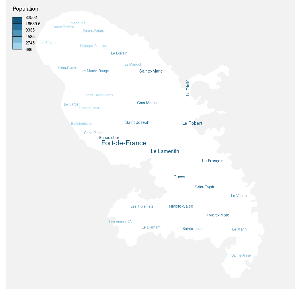
Plot a word cloud adjusted to an sf object.
wordcloudLayer(
  x,
  txt,
  freq,
  max.words = NULL,
  cex.maxmin = c(1, 0.5),
  rot.per = 0.1,
  col = NULL,
  fittopol = FALSE,
  use.rank = FALSE,
  add = FALSE,
  breaks = NULL,
  method = "quantile",
  nclass = NULL
)
Arguments
- x
an sf object, a simple feature collection (POLYGON or MULTIPOLYGON).
- txt
labels variable.
- freq
frequencies of
txt.- max.words
Maximum number of words to be plotted. least frequent terms dropped
- cex.maxmin
integer (for same size in all
txt) or vector of length 2 indicating the range of the size of the words.- rot.per
proportion words with 90 degree rotation
- col
color or vector of colors words from least to most frequent
- fittopol
logical. If true would override
rot.perfor some elements ofx- use.rank
logical. If true rank of frequencies is used instead of real frequencies.
- add
whether to add the layer to an existing plot (TRUE) or not (FALSE)
- breaks, method, nclass
additional arguments for adjusting the colors of
txt, seechoroLayer.
References
Ian Fellows (2018). wordcloud: Word Clouds.
R package version 2.6. https://CRAN.R-project.org/package=wordcloud
See also
Examples
library(sf)
mtq <- st_read(system.file("gpkg/mtq.gpkg", package = "cartography"))
#> Reading layer `mtq' from data source
#>   `/tmp/RtmpmpfIrO/temp_libpath18ee15f22a9e/cartography/gpkg/mtq.gpkg'
#>   using driver `GPKG'
#> Simple feature collection with 34 features and 7 fields
#> Geometry type: MULTIPOLYGON
#> Dimension:     XY
#> Bounding box:  xmin: 690574 ymin: 1592536 xmax: 735940.2 ymax: 1645660
#> Projected CRS: WGS 84 / UTM zone 20N
par(mar=c(0,0,0,0))
plot(st_geometry(mtq),
     col = "white",
     bg = "grey95",
     border = NA)
wordcloudLayer(
  x = mtq,
  txt = "LIBGEO",
  freq = "POP",
  add = TRUE,
  nclass = 5
)
legendChoro(
  title.txt = "Population",
  breaks = getBreaks(mtq$POP, nclass = 5, method = "quantile"),
  col = carto.pal("blue.pal", 5),
  nodata = FALSE
)