Compute the Potential Model using Parallelization

This function computes the potential model with a cutoff distance and parallel computation.

mcpotential(x, y, var, fun, span, beta, limit = 3 * span, ncl, size = 500)

Arguments

x

an sf object (POINT), the set of known observations to estimate the potentials from.

y

an sf object (POINT), the set of unknown units for which the function computes the estimates.

var

names of the variables in x from which potentials are computed. Quantitative variables with no negative values.

fun

spatial interaction function. Options are "p" (pareto, power law) or "e" (exponential). For pareto the interaction is defined as: (1 + alpha * mDistance) ^ (-beta). For "exponential" the interaction is defined as: exp(- alpha * mDistance ^ beta). The alpha parameter is computed from parameters given by the user (beta and span).

span

distance where the density of probability of the spatial interaction function equals 0.5.

beta

impedance factor for the spatial interaction function.

limit

maximum distance used to retrieve x points, in map units.

ncl

number of clusters. ncl is set to parallel::detectCores() - 1 by default.

size

mcpotential splits y in smaller chunks and dispatches the computation in ncl cores, size indicates the size of each chunks.

Value

If only one variable is computed a vector is returned, if more than one variable is computed a matrix is returned.

Examples

# \donttest{
library(sf)
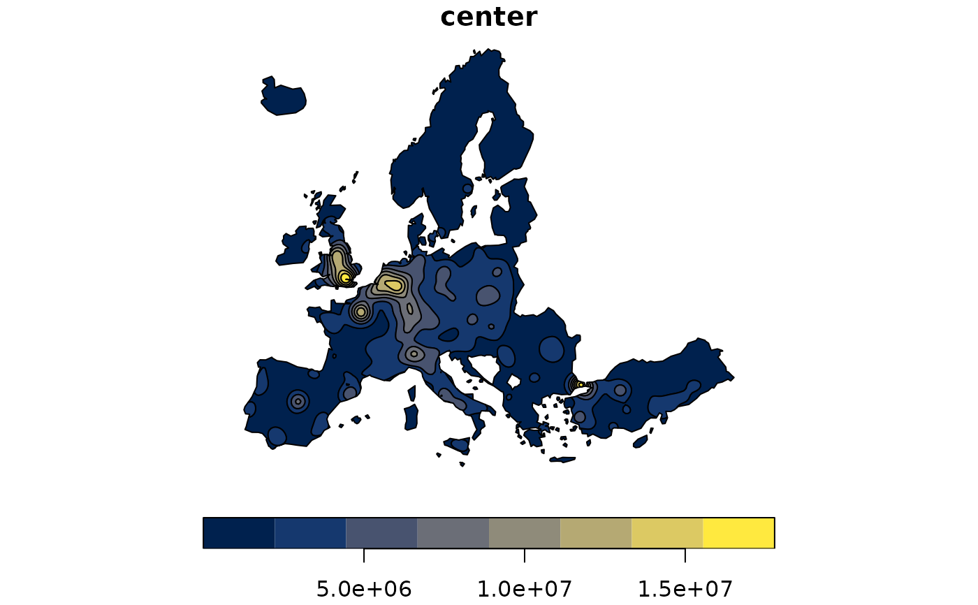
g <- create_grid(x = n3_poly, res = 20000)
pot <- mcpotential(
  x = n3_pt, y = g, var = "POP19",
  fun = "e", span = 75000, beta = 2, 
  limit = 300000, 
  ncl = 2
)
g$OUTPUT <- pot
equipot <- equipotential(g, var = "OUTPUT", mask = n3_poly)
plot(equipot["center"], pal = hcl.colors(nrow(equipot), "cividis"))

# }