Compute the Potential Model

This function computes the potential model as defined by J.Q. Stewart (1941).

potential(x, y, d, var, fun, span, beta)

Arguments

x

an sf object (POINT), the set of known observations to estimate the potentials from.

y

an sf object (POINT), the set of unknown units for which the function computes the estimates.

d

a distance matrix between known observations and unknown units for which the function computes the estimates. Row names match the row names of x and column names match the row names of y. d can contain any distance metric (time distance or euclidean distance for example).

var

names of the variables in x from which potentials are computed. Quantitative variables with no negative values.

fun

spatial interaction function. Options are "p" (pareto, power law) or "e" (exponential). For pareto the interaction is defined as: (1 + alpha * mDistance) ^ (-beta). For "exponential" the interaction is defined as: exp(- alpha * mDistance ^ beta). The alpha parameter is computed from parameters given by the user (beta and span).

span

distance where the density of probability of the spatial interaction function equals 0.5.

beta

impedance factor for the spatial interaction function.

Value

If only one variable is computed a vector is returned, if more than one variable is computed a matrix is returned.

References

STEWART, JOHN Q. 1941. "An Inverse Distance Variation for Certain Social Influences." Science 93 (2404): 89–90. doi:10.1126/science.93.2404.89 .

Examples

library(sf)
y <- create_grid(x = n3_poly, res = 200000)
d <- create_matrix(n3_pt, y)
pot <- potential(
  x = n3_pt, y = y, d = d, var = "POP19",
  fun = "e", span = 200000, beta = 2
)
y$OUTPUT <- pot
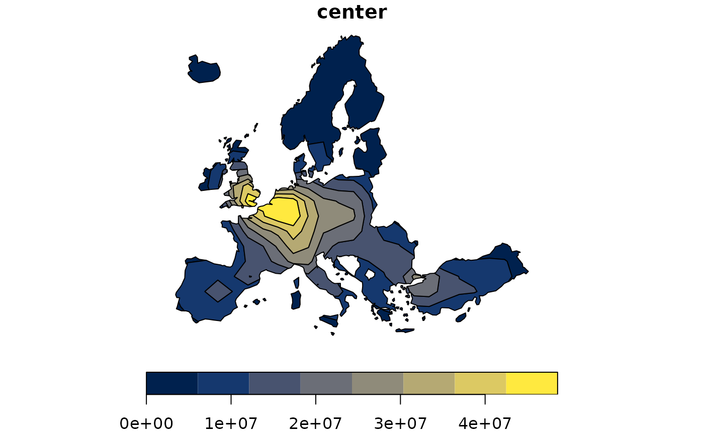
equipot <- equipotential(y, var = "OUTPUT", mask = n3_poly)
plot(equipot["center"], pal = hcl.colors(nrow(equipot), "cividis"))